Score-Based Generative Modeling
Push-forward Generative Models
Denoising Score Matching Langevin Dynamics
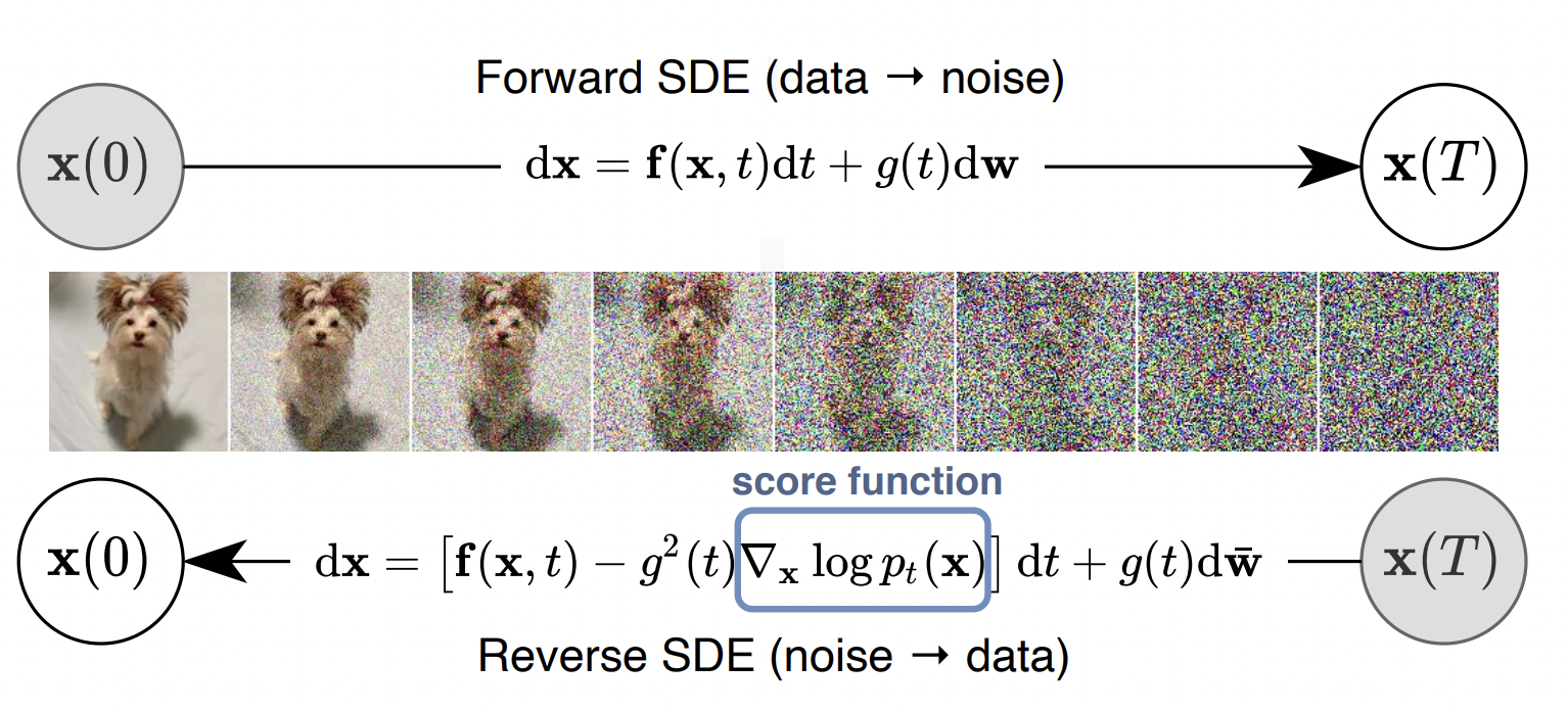
Diffusion models, also known as score-based generative models, is a new paradigm for generative modeling which exhibits state-of-the-art performance in image and audio synthesis. Such models first consider a forward stochastic process, adding noise to the data until a Gaussian distribution is reached. The model then approximates the backward process associated with this forward noising process. It can be shown, see for instance, that in order to compute the drift of the backward trajectory, the gradient of the forward logarithmic density (Stein score) must be estimated. Such an estimator is then obtained using score matching techniques and leveraging neural network techniques. At sampling time, the backward process is initialized with a Gaussian and run backward in time using the approximation of the Stein score.
Let \(p_\sigma(\tilde{\mathbf{x}} \mid \mathbf{x}):=\mathcal{N}\left(\tilde{\mathbf{x}} ; \mathbf{x}, \sigma^2 \mathbf{I}\right)\) , \(p_\sigma(\tilde{\mathbf{x}}):=\int p_{\text {data }}(\mathbf{x}) p_\sigma(\tilde{\mathbf{x}} \mid \mathbf{x}) \mathrm{d} \mathbf{x}\), where \(p_{\text {data }}(\mathbf{x})\) denotes the data distribution. Consider a sequence of positive noise scales \(\sigma_{\min }=\sigma_1<\) \(\sigma_2<\cdots<\sigma_N=\sigma_{\max }\). Typically, \(\sigma_{\min }\) is small enough such that \(p_{\sigma_{\min }}(\mathbf{x}) \approx p_{\text {data }}(\mathbf{x})\), and \(\sigma_{\max }\) is large enough such that \(p_{\sigma_{\max }}(\mathbf{x}) \approx \mathcal{N}\left(\mathbf{x} ; \mathbf{0}, \sigma_{\max }^2 \mathbf{I}\right)\). Song & Ermon (2019) propose to train a Noise Conditional Score Network (NCSN), denoted by \(\mathbf{s}_{\boldsymbol{\theta}}(\mathbf{x}, \sigma)\), with a weighted sum of denoising score matching (Vincent, 2011) objectives: \[\boldsymbol{\theta}^*=\underset{\boldsymbol{\theta}}{\arg \min } \sum_{i=1}^N \sigma_i^2 \mathbb{E}_{p_{\mathrm{data}}(\mathbf{x})} \mathbb{E}_{p_{\sigma_i}(\tilde{\mathbf{x}} \mid \mathbf{x})}\left[\left\|\mathbf{s}_{\boldsymbol{\theta}}\left(\tilde{\mathbf{x}}, \sigma_i\right)-\nabla_{\tilde{\mathbf{x}}} \log p_{\sigma_i}(\tilde{\mathbf{x}} \mid \mathbf{x})\right\|_2^2\right] .\] Given sufficient data and model capacity, the optimal score-based model \(\mathbf{s}_\theta *(\mathbf{x}, \sigma)\) matches \(\nabla_{\mathbf{x}} \log p_\sigma(\mathbf{x})\) almost everywhere for \(\sigma \in\left\{\sigma_i\right\}_{i=1}^N\). For sampling, Song & Ermon (2019) run \(M\) steps of Langevin MCMC to get a sample for each \(p_{\sigma_i}(\mathbf{x})\) sequentially: \[\mathbf{x}_i^m=\mathbf{x}_i^{m-1}+\epsilon_i \mathbf{s}_{\boldsymbol{\theta}^*}\left(\mathbf{x}_i^{m-1}, \sigma_i\right)+\sqrt{2 \epsilon_i} \mathbf{z}_i^m, \quad m=1,2, \cdots, M,\] where \(\epsilon_i>0\) is the step size, and \(\mathbf{z}_i^m\) is standard normal. The above is repeated for \(i=N, N-\) \(1, \cdots, 1\) in turn with \(\mathbf{x}_N^0 \sim \mathcal{N}\left(\mathbf{x} \mid \mathbf{0}, \sigma_{\max }^2 \mathbf{I}\right)\) and \(\mathbf{x}_i^0=\mathbf{x}_{i+1}^M\) when \(i<N\). As \(M \rightarrow \infty\) and \(\epsilon_i \rightarrow 0\) for all \(i, \mathbf{x}_1^M\) becomes an exact sample from \(p_{\sigma_{\min }}(\mathbf{x}) \approx p_{\text {data }}(\mathbf{x})\) under some regularity conditions.
Estimating Scores using SDE
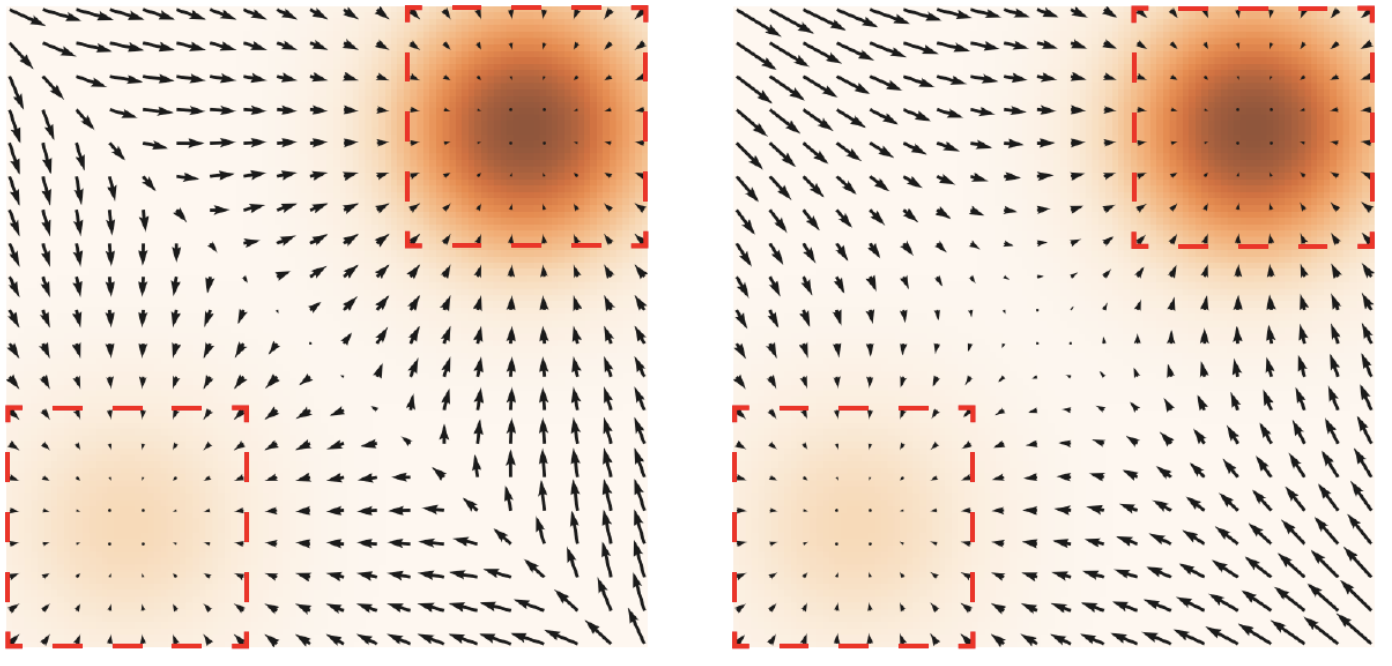
Figure: (left) \(\nabla_{\mathbf{x}} \log p_{\text {data }}(\mathbf{x})\). (right) \(\mathbf{s}_{\boldsymbol{\theta}}(\mathbf{x})\) The data density \(p_{\text {data }}(\mathbf{x})\) is encoded using an orange colormap: darker color implies higher density. Red rectangles highlight regions where \(\nabla_{\mathbf{x}} \log p_{\text {data }}(\mathbf{x}) \approx \mathbf{s}_{\boldsymbol{\theta}}(\mathbf{x})\).
The score of a distribution can be estimated by training a score-based model on samples with score matching. To estimate \(\nabla_{\mathbf{x}} \log p_t(\mathbf{x})\), we can train a time-dependent score-based model \(\mathbf{s}_{\boldsymbol{\theta}}(\mathbf{x}, t)\) via a continuous generalization: \[ \boldsymbol{\theta}^*=\underset{\boldsymbol{\theta}}{\arg \min } \mathbb{E}_t\left\{\lambda(t) \mathbb{E}_{\mathbf{x}(0)} \mathbb{E}_{\mathbf{x}(t) \mid \mathbf{x}(0)}\left[\left\|\mathbf{s}_{\boldsymbol{\theta}}(\mathbf{x}(t), t)-\nabla_{\mathbf{x}(t)} \log p_{0 t}(\mathbf{x}(t) \mid \mathbf{x}(0))\right\|_2^2\right]\right\} . \] Here \(\lambda:[0, T] \rightarrow \mathbb{R}_{>0}\) is a positive weighting function, \(t\) is uniformly sampled over \([0, T]\), \(\mathbf{x}(0) \sim p_0(\mathbf{x})\) and \(\mathbf{x}(t) \sim p_{0 t}(\mathbf{x}(t) \mid \mathbf{x}(0))\). With sufficient data and model capacity, score matching ensures that the optimal solution to Eq. (7), denoted by \(\mathbf{s}_{\boldsymbol{\theta}^*}(\mathbf{x}, t)\), equals \(\nabla_{\mathbf{x}} \log p_t(\mathbf{x})\) for almost all \(\mathbf{x}\) and \(t\). As in SMLD and DDPM, we can typically choose \(\lambda \propto 1 / \mathbb{E}\left[\left\|\nabla_{\mathbf{x}(t)} \log p_{0 t}(\mathbf{x}(t) \mid \mathbf{x}(0))\right\|_2^2\right]\).
Push-forward generative models
Score-Based Generative Modeling (SGM) is a recently developed approach to probabilistic generative modeling that exhibits state-of-the-art performance on several audio and image synthesis tasks. Progressively applying Gaussian noise transforms complex data distributions to approximately Gaussian. Reversing this dynamic defines a generative model. When the forward noising process is given by a Stochastic Differential Equation (SDE), Song et al. (2021) demonstrate how the time inhomogeneous drift of the associated reverse-time SDE may be estimated using score-matching. A limitation of this approach is that the forward-time SDE must be run for a sufficiently long time for the final distribution to be approximately Gaussian while ensuring that the corresponding time-discretization error is controlled.
Theorem 1. Let \(g: \mathbb{R}^p \rightarrow \mathbb{R}^d\) be a Lipschitz function with Lipschitz constant \(\operatorname{Lip}(g)\). Then for any Borel set \(\mathrm{A} \in \mathcal{B}\left(\mathbb{R}^d\right)\), \[\operatorname{Lip}(g)\left(g_{\#} \mu_p\right)^{+}(\partial \mathrm{A}) \geq \varphi\left(\Phi^{-1}\left(g_{\#} \mu_p(\mathrm{~A})\right)\right)\] where \(\varphi(x)=(2 \pi)^{-1 / 2} \exp \left[-x^2 / 2\right]\) and \(\Phi(x)=\int_{-\infty}^x \varphi(t) \mathrm{d} t\). In addition, we have that for any \(r \geq 0\) \[g_{\#} \mu_p\left(\mathrm{~A}_r\right) \geq \Phi\left(r / \operatorname{Lip}(g)+\Phi^{-1}\left(g_{\#} \mu_p(\mathrm{~A})\right)\right) \text {. }\]
Let \(\nu\) be a probability measure on \(\mathbb{R}\) with density w.r.t. the Lesbesgue measure and such that \(\operatorname{supp}(\nu)=\mathbb{R}\). Assume that there exists \(g: \mathbb{R}^p \rightarrow \mathbb{R}\) Lipschitz such that \(\nu=g_{\#} \mu_p\). Let us denote \(T_{\mathrm{OT}}=\Phi_\nu^{-1} \circ \Phi\) the Monge map between \(\mu_1\) and \(\nu\), where \(\Phi_\nu\) is the cumulative distribution function of \(\nu\). Then we have \(\operatorname{Lip}(g) \geq \operatorname{Lip}\left(T_{\mathrm{OT}}\right)\).
Poisson Flow Generative Models
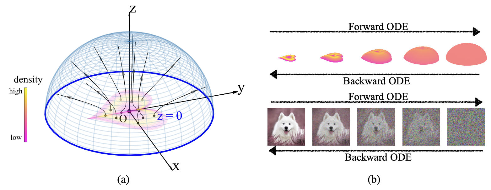
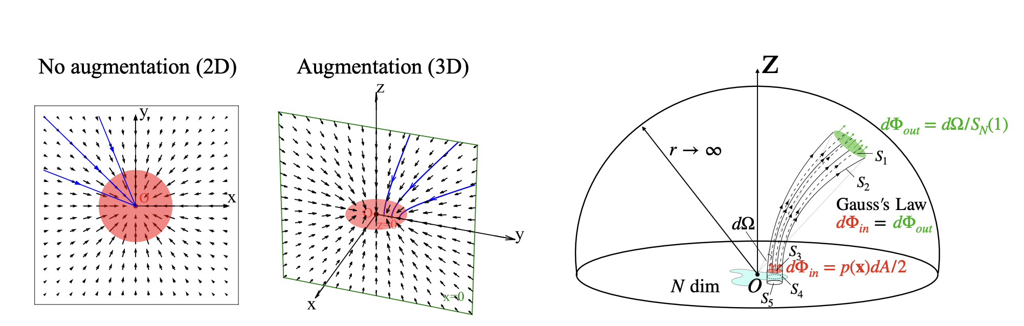
The Poisson flow generative model (PFGM) maps a uniform distribution on a high-dimensional hemisphere into any data distribution. They interpret the data points as electrical charges on the \(\mathrm{z}=\) 0 hyperplane in a space augmented with an additional dimension z, generating a high-dimensional electric field (the gradient of the solution to Poisson equation). They prove that if these charges flow upward along electric field lines, their initial distribution in the \(\mathrm{z}=0\) plane transforms into a distribution on the hemisphere of radius \(r\) that becomes uniform in the \(r \rightarrow \infty\) limit. To learn the bijective transformation, they estimate the normalized field in the augmented space.
We wish to generate samples \(\mathbf{x} \in \mathbb{R}^N\) from a distribution \(p(\mathbf{x})\) supported on a bounded region. We may set the source \(\rho(\mathbf{x})=p(\mathbf{x}) \in \mathcal{C}^0\) and compute the resulting gradient field \(\mathbf{E}(\mathbf{x})\). Since \(-\mathbf{E}(\mathbf{x})\) points towards sources, the backward ODE \(d \mathbf{x} / d t=-\mathbf{E}(\mathbf{x})\) will take samples close to the sources. One may naively hope that the backward ODE is a generative model that recovers \(p(\mathbf{x})\). Unfortunately, the backward ODE has the problem of mode collapse. We illustrate this phenomenon with a 2D uniform disk. The reverse Poisson field \(-\mathbf{E}(\mathbf{x})\) on the 2D \((x, y)\)-plane points towards the center of the disk \(O\) (Fig. 2(a) left), so all particle trajectories will eventually hit \(O\). If we instead add an additional dimension \(z\), particles can hit different points on the disk and faithfully recover the data distribution.
Consequently, instead of solving the Poisson equation \(\nabla^2 \varphi(\mathbf{x})=-p(\mathbf{x})\) in the original data space, we solve the Poisson equation in an augmented space \(\tilde{\mathbf{x}}=(\mathbf{x}, z) \in \mathbb{R}^{N+1}\) with an additional variable \(z \in \mathbb{R}\). We augment the training data \(\tilde{\mathbf{x}}\) in the new space by setting \(z=0\) such that \(\tilde{\mathbf{x}}=(\mathbf{x}, 0)\). As a consequence, the data distribution in the augmented space is \(\tilde{p}(\tilde{\mathbf{x}})=p(\mathbf{x}) \delta(z)\), where \(\delta\) is the Dirac delta function. The Poisson field by solving the new Poisson equation \(\nabla^2 \varphi(\tilde{\mathbf{x}})=-\tilde{p}(\tilde{\mathbf{x}})\) has an analytical form: \[ \forall \tilde{\mathbf{x}} \in \mathbb{R}^{N+1}, \mathbf{E}(\tilde{\mathbf{x}})=-\nabla \varphi(\tilde{\mathbf{x}})=\frac{1}{S_N(1)} \int \frac{\tilde{\mathbf{x}}-\tilde{\mathbf{y}}}{\|\tilde{\mathbf{x}}-\tilde{\mathbf{y}}\|^{N+1}} \tilde{p}(\tilde{\mathbf{y}}) d \tilde{\mathbf{y}} \] The associated forward/backward ODEs of the Poisson field are \(d \tilde{\mathbf{x}} / d t=\mathbf{E}(\tilde{\mathbf{x}}), d \tilde{\mathbf{x}} / d t=-\mathbf{E}(\tilde{\mathbf{x}})\). Intuitively, theses ODEs uniquely define trajectories of particles between the \(z=0\) hyperplane and an enclosing hemisphere. In the following theorem, we show that the backward ODE defines a transformation between the uniform distribution on an infinite hemisphere and the data distribution \(\tilde{p}(\tilde{\mathbf{x}})\) in the \(z=0\) plane.
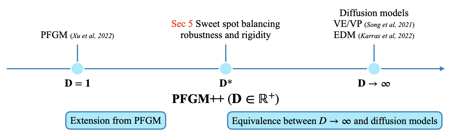
PFGM++
While PFGM consider the electric field in a \(N+1\)-dimensional augmented space, we augment the data \(\mathbf{x}\) with \(D\)-dimensional variables \(\mathbf{z}=\left(z_1, \ldots, z_D\right)\), i.e., \(\tilde{\mathbf{x}}=(\mathbf{x}, \mathbf{z})\) and \(D \in \mathbb{Z}^{+}\). Similar to the \(N+1\)-dimensional electric field, the electric field at the augmented data \(\tilde{\mathbf{x}}=(\mathbf{x}, \mathbf{z}) \in \mathbb{R}^{N+D}\) is: \[ \mathbf{E}(\tilde{\mathbf{x}})=\frac{1}{S_{N+D-1}(1)} \int \frac{\tilde{\mathbf{x}}-\tilde{\mathbf{y}}}{\|\tilde{\mathbf{x}}-\tilde{\mathbf{y}}\|^{N+D}} p(\mathbf{y}) d \mathbf{y} \]
Analogous to the theoretical results presented in PFGM, with the electric field as the drift term, the ODE \(d \tilde{\mathbf{x}}=\mathbf{E}(\tilde{\mathbf{x}}) \mathrm{d} t\) defines a surjection from a uniform distribution on an infinite \(\mathrm{N}+\mathrm{D}\)-dim hemisphere and the data distribution on the \(\mathrm{N}\) \(\operatorname{dim} \mathbf{z}=\mathbf{0}\) hyperplane. However, the mapping has \(S O(D)\) symmetry on the surface of \(D\)-dim cylinder \(\sum_{i=1}^D z_i^2=r^2\) for any positive \(r\). We provide an illustrative example at the bottom of Fig. \(2(D=2, N=1)\), where the electric flux emitted from a line segment (red) has rotational symmetry through the ring area (blue) on the \(z_1^2+z_2^2=r^2\) cylinder. Hence, instead of modeling the individual behavior of each \(z_i\), it suffices to track the norm of augmented variables \(r(\tilde{\mathbf{x}})=\|\mathbf{z}\|_2-\) due to symmetry. Specifically, note that \(\mathrm{d} z_i=\mathbf{E}(\tilde{\mathbf{x}})_{z_i} \mathrm{~d} t\), and the time derivative of \(r\) is
\[ \begin{aligned} \frac{\mathrm{d} r}{\mathrm{~d} t} & =\sum_{i=1}^D \frac{z_i}{r} \frac{\mathrm{d} z_i}{\mathrm{~d} t}=\int \frac{\sum_{i=1}^D z_i^2}{S_{N+D-1}(1) r\|\tilde{\mathbf{x}}-\tilde{\mathbf{y}}\|^{N+D}} p(\mathbf{y}) \mathrm{d} \mathbf{y} \\ & =\frac{1}{S_{N+D-1}(1)} \int \frac{r}{\|\tilde{\mathbf{x}}-\tilde{\mathbf{y}}\|^{N+D}} p(\mathbf{y}) \mathrm{d} \mathbf{y} \end{aligned} \]
Henceforth we replace the notation for augmented data with \(\tilde{\mathbf{x}}=(\mathbf{x}, r)\) for simplicity. After the symmetry reduction, the field to be modeled has a similar form except that the last \(D\) sub-components \(\left\{\mathbf{E}(\tilde{\mathbf{x}})_{z_i}\right\}_{i=1}^D\) are condensed into a scalar \(E(\tilde{\mathbf{x}})_r=\frac{1}{S_{N+D-1}(1)} \int \frac{r_r}{\|\tilde{\mathbf{x}}-\tilde{\mathbf{y}}\|^{N+D}} p(\mathbf{y}) \mathrm{d} \mathbf{y}\). Therefore, we can use the physically meaningful \(r\) as the anchor variable in the ODE \(\mathrm{d} \mathbf{x} / \mathrm{d} r\) by change-of-variable: \[ \frac{\mathrm{d} \mathbf{x}}{\mathrm{d} r}=\frac{\mathrm{d} \mathbf{x}}{\mathrm{d} t} \frac{\mathrm{d} t}{\mathrm{~d} r}=\mathbf{E}(\tilde{\mathbf{x}})_{\mathbf{x}} \cdot E(\tilde{\mathbf{x}})_r^{-1}=\frac{\mathbf{E}(\tilde{\mathbf{x}})_{\mathbf{x}}}{E(\tilde{\mathbf{x}})_r} \]
Indeed, the ODE \(\mathrm{d} \mathbf{x} / \mathrm{d} r\) turns the aforementioned surjection into a bijection between an easy-to-sample prior distribution on the \(r=r_{\max }\) hyper-cylinder \({ }^2\) and the data distribution on \(r=0\) (i.e., \(\mathbf{z}=\mathbf{0}\) ) hyperplane. The following theorem states the observation formally:
Theorem 1. Assume the data distribution \(p \in \mathcal{C}^1\) and \(p\) has compact support. As \(r_{\max } \rightarrow \infty\), for \(D \in \mathbb{R}^{+}\), the \(O D E \mathrm{~d} \mathbf{x} / \mathrm{d} r=\mathbf{E}(\tilde{\mathbf{x}})_{\mathbf{x}} / E(\tilde{\mathbf{x}})_r\) defines a bijection between \(\lim _{r_{\max } \rightarrow \infty} p_{r_{\max }}(\mathbf{x}) \propto \lim _{r_{\max } \rightarrow \infty} r_{\text {max }}^D /\left(\|\mathbf{x}\|_2^2+r_{\text {max }}^2\right)^{\frac{N+D}{2}}\) when \(r=r_{\max }\) and the data distribution \(p\) when \(r=0\).
Diffusion models generate samples by simulating ODE/SDE involving the score function \(\nabla_{\mathbf{x}} \log p_\sigma(\mathbf{x})\) at different intermediate distributions \(p_\sigma\), where \(\sigma\) is the standard deviation of the Gaussian kernel. In this section, we show that both sampling and training schemes in diffusion models are equivalent to those in \(D \rightarrow \infty\) case under the PFGM++ framework. To begin with, we show that the electric field in PFGM++ has the same direction as the score function when \(D\) tends to infinity, and their sampling processes are also identical.
Theorem. Assume the data distribution \(p \in \mathcal{C}^1\). Consider taking the limit \(D \rightarrow \infty\) while holding \(\sigma=r / \sqrt{D}\) fixed. Then, for all \(\mathbf{x}\), \[ \lim _{\substack{D \rightarrow \infty \\ r=\sigma \sqrt{D}}}\left\|\frac{\sqrt{D}}{E(\tilde{\mathbf{x}})_r} \mathbf{E}(\tilde{\mathbf{x}})_{\mathbf{x}}-\sigma \nabla_{\mathbf{x}} \log p_{\sigma=r / \sqrt{D}}(\mathbf{x})\right\|_2=0 \]
Further, given the same initial point, the trajectory of the PFGM++ ODE matches the diffusion ODE in the same limit.
See:
- Score-Based Generative Modeling through Stochastic Differential Equations
- Can Push-forward Generative Models Fit Multimodal Distributions?
-
See Automatic Symmetry Discovery with Lie Algebra Convolutional Network for a good intro. ↩︎