Lie Groups and Lie Algebras
Introduction to Continuous Groups
Lie Groups
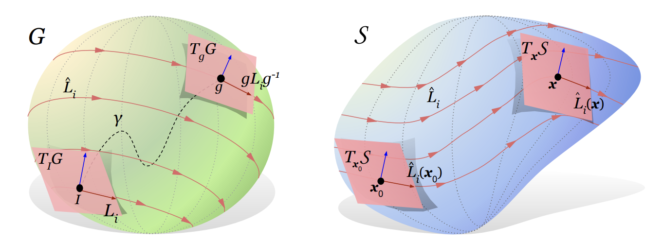
Figure 1: Lie group and Lie algebra: Illustration of the group manifold of a Lie group G (left). The Lie algebra 𝔤 = TIG is the tangent space at the identity I.Li are a basis for TIG. If G is connected, ∀g ∈ G there exist paths like γ from I to g and g can be written as a path-ordered integral g = Pexp [∫γdtiLi]. Base space Right is a schematic of the base space 𝒮 as a manifold. The lift x = gx0 takes x ∈ 𝒮 to g ∈ G, and maps the tangent spaces Tx𝒮 → TgG. Each Lie algebra basis Li ∈ 𝔤 = TIG generates a vector field L̂i on the tangent bundle TG via the pushforward L̂i(g) = gLig−1. Via the lift, Li also generates a vector field L̂i = L̂iα(x)∂α = [gLix0]α∂α.
A Lie group G is a smooth manifold together with a distinguished element e ∈ G, and smooth maps multiplication: G × G → G and inverse: G → G (this map is required to be a diffeomorphism) such that G is a group with these operations and with e being the identity element. A morphism of Lie groups is a group homomorphism f : G → H which is also a smooth map.
The tangent space g at the identity element of a Lie group G has a rule of composition (X, Y) → [X, Y] derived from the bracket operation on the left invariant vector fields on G. The vector space g with this rule of composition is called the Lie algebra of G. The structures of g and G are related by the exponential mapping exp: g → G which sends straight lines through the origin in g onto one-paramater subgroups of G. Although the structure of g is determined by an arbitrary neighborhood of the identity element of G, the exponential mapping sets up a far-reaching relationship between g and the group G in the large.
More generally, let a be a vector space over a field K (of characteristic 0). The set a is called a Lie algebra over K if there is given a rule of composition (X, Y) → [X, Y] in a which is bilinear and satisfies (a) [X, X] = 0 for all X ∈ a; (b) [X, [Y, Z]] + [Y, [Z, X]] + [Z, [X, Y]] = 0 for all X, Y, Z ∈ a. The identity (b) is called the Jacobi identity. The Lie algebra of G above is clearly a Lie algebra over R. If a is a Lie algebra over K and X ∈ a, the linear transformation Y → [X, Y] of a is denoted by ad X (or adaX when a confusion would otherwise be possible). Let 𝔟 and c be two vector subspaces of a. Then [b, c] denotes the vector subspace of a generated by the set of elements [X, Y] where X ∈ 𝔟, Y ∈ c. A vector subspace b of a is called a subalgebra of a if [b, b] ⊂ b and an ideal in a if [b, a] ⊂ b. If b is an ideal in a then the factor space a/b is a Lie algebra with the bracket operation inherited from a. Let a and b be two Lie algebras over the same field K and σ a linear mapping of a into b. The mapping σ is called a homomorphism if σ([X, Y]) = [σX, σY] for all X, Y ∈ 𝔞. If σ is a homomorphism then σ(a) is a subalgebra of b and the kernel σ−1{0} is an ideal in a. If σ−1{0}= {0}, then σ is called an isomorphism of a into b. An isomorphism of a Lie algebra onto itself is called an automorphism. If a is a Lie algebra and b, c subsets of a, the centralizer of b in c is {X ∈ 𝔠 : [X, b] = 0}. If b ∣ ca is a subalgebra, its normalizer in a is 𝔫 = {X ∈ 𝔞 : [X, 𝔟] ⊂ 𝔟}; 𝔟 is an ideal in n.
Examples:
(ℝn, +, 0).
(ℂ*, x, 1).
(S1, x, 1). Moreover, f : ℝ → S1 given by f(x) = eix is a Lie group morphism.
(GL(n, ℝ), x, I).
$S U(2)=\left(\begin{array}{cc}a & b \\ -\bar{b} & \bar{a}\end{array}\right)$ such that |a|2 + |b|2 = 1. That is, SU(2) is homeomorphic to S3 (and hence can be made into a smooth manifold which is in fact a smooth submanifold of ℝ4 ). It is easy to see that the group operations are smooth.
SL(n, ℝ) is a Lie group of dimension n2 − 1.
SO(n), O(n), SU(n), U(n) are Lie groups. For instance, {O(n) ⊂ ℝn2 ∣ AAT = I}. We want to use the Inverse Function Theorem (IFT). So consider the smooth function F(A) = ATA defined on the open subset of invertible matrices. Its derivative is F′(B) = ATB + BTA = (BTA)T + BTA whose kernel consists of skew-symmetric matrices C of the type C = ATB. Thus define B = AC. Thus the rank is a constant. The constant rank theorem implies that F−1(I) is a manifold of dimension $n^2-\frac{n(n-1)}{2}$. The multiplication and inverse operations are inherited from M(n, ℝ) and hence smooth.
It turns out that the manifold G = ℝ × ℝ × S1 given a group structure as (x1, x2, u1).(x2, y2, u2) = (x1+x2, y1+y2 , eix1y2 u1u2) is a Lie group but not a matrix Lie group! That is, it is not a Lie subgroup (embedded submanifold such that the inclusion is a group homomorphism - this is usually called a closed Lie subgroup whereas the term Lie subgroup is usually reserved for immersed submanifolds, but we shall not do so in this set of lectures) of GL(n, ℝ) for any n.
Why should we care?
Discrete case: Suppose we shuffle cards in some way (I know of only one way - the overhand shuffle). We want to know how many times one must do it so that the cards become sufficiently random. This can be modeled as an operation (convolution) of probability distributions on Sn. More generally, the study of probability distributions on groups leads to interesting applications in real life.
Continuous case: A continuous version of the problem above in a higher-dimensional (sphere instead of circle) case is as follows: Consider the Hydrogen atom. In quantum mechanics, the only “energy levels” of the Hydrogen atom correspond to the spectrum of an operator which is simply the Laplacian plus C/r. So naively speaking, we want to find the “eigenvalues” of such an operator. We notice that there is a rotational symmetry. So we can simply “diagonalise” all rotations (NOT possible because of non-commutativity) and hope that the “eigenvectors” of the hydrogen atom can be computed by restricting ourselves to the “eigenspaces” (actually irreducible representations) of the rotations. The collection of all rotations form an infinite group (SO (3)).
Matrix Lie groups
Definition: A Lie subgroup of GL(n,R) is called a matrix Lie group.
Example: $H:=\left\{\left[\begin{array}{lll}1 & a & b \\ 0 & 1 & c \\ 0 & 0 & 1\end{array}\right] \in M(3, \mathbb{R})\right\}$ is a Lie group called the Heisenberg group. Note that, $$\Phi\left(\left[\begin{array}{lll} 1 & a & b \\ 0 & 1 & c \\ 0 & 1 & 1 \end{array}\right]\right):=\left(a, c, e^{\sqrt{-1} b}\right)$$ is a Lie homomorphism.
Definition: Let \(M\) be a smooth manifold and \(G\) a Lie group. A left action of \(G\) on \(M\) is a smooth map, \[ (\cdot): G \times M \rightarrow M \] such that, \[ \begin{aligned} & g_1\cdot(g_2\cdot(p)=(g_1g_2) \cdot p \\ & e \cdot p=p \end{aligned} \] Definition: A representation of a Lie group \(G\) on finite dimensional vector space \(V\) is a Lie group action \(G \times V \rightarrow V\), such that \(g \cdot v \rightarrow v\) is linear, ie. \(f\) a smooth Lie map, \[ \rho: G \rightarrow G L(V). \]
Examples:
\(G L(n, \mathbb{R})\) acts transitively on \(r\)-dimensional subspaces of \(\mathbb{R}^n\), and the coset apace can be given a smooth structure, called the Grassmanian.
If \(G \rightarrow M\), then \(G\) acts on \(C^{\infty}(M)\) as follows: \[ f \in C^{\infty}(M) \rightarrow g \cdot f:=f \circ g^{-1} \]
Likewise, if \(x \in X(M)\), and \(G \rightarrow M\), then \(G \rightarrow X(M)\) given as: \[ (g \cdot X)_p:=\left.D g^{-1}\right|_{g(p)}\left(X_{g(p)}\right) \] If \(w\) is a 1-form, then, \[ (g \cdot \omega)_p\left(x_p\right):=\omega_{g^{-1}(p)}\left(\left(g^{-1}\right)_*\left(x_p\right)\right) \]
- Suppose \(P \in M\) is a fixed point of a Lie group action on \(M\), then we get that the map \(g \mapsto\left(g_*\right)_p \in G L\left(T_p M\right)\) is a representation of \(G\).
Theorem 1. Let G be a (possibly disconnected) Lie group. Let G0 be the connected component of identity. Then G0 is a normal Lie subgroup of G. The quotient group G/G0 is discrete.
Unless specified otherwise, we will now assume that G is connected. An example of a connected Lie group is GL(n, ℂ) : Let g be such a matrix. Let g = PJP−1 where J is the Jordan canonical form. It is easy to see that J can be connected to identity (and hence so can g).
Matrix Exponentials
There are two reasons to care about matrix exponentials.
1. The constant rank theorem proves that \(S O(3)\) is a Lie group, but we want a more concrete description of rotations. Suppose we consider an infinitesimal rotation near the identity, i.e., \(A=I+B\). Now \((I+B)(I+B)^T=I\) and hence \(B+B^T \approx 0\). Conversely, if \(B+B^T \approx 0\), then \((I+B)\left(I+B^T\right) \approx I\). To make the approximation better, we can rotate by “half-angles”, i.e., \((I+B / 2)^2\left(I+B^T / 2\right)^2=I+B^2 / 2+O\left(B^3\right)\). This motivates us to study \(\lim _{N \rightarrow \infty}(I+B / N)^N\).
2. Consider the system of ODE: \(\frac{d v}{d t}=A v\) where \(A\) is a matrix. One would naively expect the solution to be \(e^{A t} v_0\) if \(e^{A t}\) is suitably defined. (In fact, for certain systems, this is the Schrödinger equation and hence the matrix exponential plays a starring role in quantum computing). Definition: For any complex matrix \(X\), define \(e^X:=I+X+X^2 / 2 !+\ldots\) This definition is valid because \(1+\|X\|+\ldots\) (Hilbert-Schmidt) converges and \(\left|X_{i j}\right| \leq\|X\|\).
We begin now by asking can the group structure be recovered similarly: if so , one can work with skew symmetric matrices instead of \(O(n)\). Observe, for \(x, y\) skew symmetric, \(e^x, e^y \in O(n)\), and, \[ \begin{aligned} & e^{t x} \cdot e^{t y}=\left(I+t x+\frac{t^2 x^2}{2 !}+\cdots\right)\left(I+t y+\frac{t^2 y^2}{2 !}+\cdots\right) \\ & =I+t(x+y)+t^2 / 2\left(x^2+y^2+2 x y\right)+O\left(t^3\right) \\ & =I+t(x+y)+t^2 / 2(x+y)^2+t^2 / 2[x, y]+O\left(t^3\right) \\ & \approx e^{t(x+y)+t^2 / 2[x, y]}+O\left(t^3\right) \\ & \end{aligned} \] For recovering group operations one needs to study the commutator. That would facilitate “infinitesimal” recovery of those operations. We therefore ask analogies for skew-symmetric matrices, matrix exponential, and commutations for an abstract Lie group (instead of \(O(n)\)).
How does one compute \(e^X\) in any concrete case? A “theoretical” (that is, not a very efficient algorithm) is to simply take the Jordan canonical form \(X=P J P^{-1}\) and write \(e^X=P e^J P^{-1}\). Now to compute \(e^J\), one simply needs to do it for every Jordan block. Each such block is of the form \(B=\lambda I+N\) where \(N\) is upper-triangular and hence nilpotent. \(I\) and \(N\) commute and hence \(e^B=e^\lambda e^N\) which can be computed quickly. This algorithm is not very efficient (because it needs computation of the eigenvalues and eigenvectors). In many cases \((I+X / N)^N\) can be better. Using a power series, we can define the matrix Logarithm: \(\ln (A):=\sum_{m=1}^{\infty}(-1)^{m+1} \frac{(A-I)^m}{m}\) whenever the series converges (for instance, when \(\|A-I\|<1\) ).
For recovering group operations one needs to study the commutator. That would facilitate “infinitesimal” recovery of those operations. We therefore ask analogues for skew-symmetric matrices, matrix exponential, and commutations for an abstract Lie group (instead of \(O(n)\)).
Here we list out analogies for things done in the case when the Lie group \(G=O(n)\):
The act of taking limits \(t x \rightarrow 0\), can be done with the help of \(T_{e}G\).
The commutator satisfies:
- Bilinearity: $[a x+b y, z] = a[x, z]+b[y, z]$
- Anticommutativity: \([x, y]=-[y, x]\)
- Jacobi Identity: $[x,[y, z]]+[y,[z, x]]+[z,[x, y]] = 0$, for all scalars $a, b$ in $F$ and all elements $x, y, z$ in $\mathfrak{g}$.
- Matrix exponential features as means to solve linear differential equation \(d v / d t=X v\). The analogue for this would be finding the flow of appropriate vector field.
Invariant vector fields
A vector field on \(G\) is left-invariant if it satisfies \(L_{g}\cdot X=X\) i.e., \[ \left.\left(L_g\right)_*\right|_{g^{-1}(p)}\left(X_{g^{-1}(p)}\right)=\left(L_g X\right)_p=X_p \]
Let \(v \in T_e G\), set \(X_g:=\left.\left(\mathcal{L}_g\right)_*\right|_e(v)\), then by chain rule \(X\) is a left invariant vector field. The map, \[ \begin{aligned} & T_e G \longrightarrow \begin{array}{l} \text { left invariant } \\ \text { vector fields on } G \end{array} \\ & v \longrightarrow x_g=\left.\left(L_g\right)_*\right|_e(v) \end{aligned} \] is an isomorphism.
Definition: The commutator \([\cdot, \cdot]\) on \(g=T_e G\) is defined as, \[ [v, w]=\left[x_v, x_w\right]_e \] where \(X_v, X_w\) are left-invariant extension of \(v, w\). This \([\cdot, \cdot]\) makes \(g\) into a Lie algebra.
Definition: Let \(x, y\) be vector fields on \(M\), then,
\[ [x, y](f):=x(y(f))-y(x(f)) \quad\left(\forall f \in C^{\infty}(M)\right) \text {. } \]
(this clearly is smooth, for \([X, Y](f) \in C^{\infty}(M)\), as \(X(f), y(f)\) \(\left.\in C^{\infty}(M)\right)\).
\[ \begin{aligned} \text{If}, X=\sum_k x^k \partial / \partial x^k, Y=\sum_k y^k \partial / \partial x^k, \text { then } \\ {[x, y]=\sum_i\left(\sum_j\left(x^j \frac{\partial y^i}{\partial x^j}-y^j \frac{\partial x^i}{\partial x^j}\right)\right) \partial / \partial x_i } \end{aligned} \]
(one can check this by evaluating \([X, Y]\left(x_i\right)\) ).
Remark: Vector fields are relevant for manifolds because their flows can give us a family of diffeomorphisms. In fact, for compact connected manifolds, any two points can be exchanged by a diffeomorphism.
One-parameter subgroup
Theorem: Let \(G\) be the Lie group, \(g=T_e G\), and \(v \in g\). Then \(\exists!\) a Lie group morphism \(\gamma_\nu: \mathbb{R} \rightarrow G\) such that \(\gamma_\nu^{\prime}(0)=\nu\). This map is called the one-parameter subgroup corresponding to \(\nu\).
Proof: Extend \(v\) uniquely to a left invariant vector field \(V\). We shall establish uniqueness: Let \(\gamma_v(t)\) be a one parameter subgroup. Choose coordinates such that,
\[ \begin{aligned} \gamma_v^{\prime}(t) & \left.=\sum_i \gamma_v^{\prime}(t)^{(i)} \partial / \partial x_i\right. \\ \gamma_v^{\prime}(t)^{(i)} & =\lim _{h \rightarrow 0} \frac{\gamma_v(t+h)^{(i)}-\gamma_v(t)^{(i)}}{h} \\ & =\lim _{h \rightarrow 0} \frac{L_{\gamma_v(t)}\left(\gamma_v(h)\right)^{(i)}-L_{\gamma_v(t)}\left(\gamma_v(0)\right)^{(i)}}{h} \end{aligned} \]
By Chain rule,
\[ \begin{gathered} {\left[\left(L_{\gamma_v(t)}\right)_*\left(\gamma_v^{\prime}(0)\right)\right]^{(i)}=\left[\left(L_{\gamma_v(t)}\right)_*(v)\right]^{(i)}=\left(V\left(\gamma_v(t)\right)\right)^{(i)}} \\ \Rightarrow \frac{d \gamma_v}{d t}=V(\gamma(t)) \\ \gamma_v(0)=e \end{gathered} \]
Thus, \(\gamma_v(t)\) is unique (by uniqueness of ODEs).
Let \(G\) be a Lie group and \(g\) be its Lie algebra. Then,
\[ \begin{aligned} & \exp : g \mapsto G \\ & \exp (v):=\gamma_v(1) \end{aligned} \]
is called the exponential map.
Remark: On a compact Lie group, the exponential form coming from Riemannian geometry coincides with the map above.
Examples:
- \(G=S^{1}, g=T_e S^{\prime}=\mathbb{R}\). Given \(v \in g\),
\[ \left.\left(X_v\right)\right|_{e^{i \theta}}=e^{i \theta}(v) \] In particular its interval curve is given by \(e^{i v t}\) ( \(v\) seen as complex number).
- More generally, \(G=G L(n, \mathbb{R})\), then \(g l(n, \mathbb{R})=M(n, \mathbb{R})\).
Given, \(A \in g l(n, \mathbb{R})\), the invariant vector field for \(A\) is,
\[ V(g):=gA \] Since, \(\left(L_g\right)_*(A)=gA\), the integral curve satisfies, \[ \begin{aligned} \frac{d \gamma_A}{d t} & =\gamma_A(t) A \\ \gamma_A(0) & =I_d \\ \Rightarrow \gamma_A(t) & =e^{A t} . \end{aligned} \]
Properties:
\(\exp\) is a smooth map (by ODE theory).
\(\operatorname{exp}(0)=e,(\exp )_*(0)=I_d\).
By Inverse Function Theorem, exp is a local diffeomorphism near 0.
\(\exp ((t+s) x)=\exp (t x) \exp (s x)\).
If \(\phi\) is a Lie group morphism, then, \[ \exp \left(\phi_*(v)\right)=\phi(\exp (v)). \]
\(X \exp (y) X^{-1}=\exp \left(\left(A_X\right)_*(y)\right) \text {, where } A_X(g)=X g X^{-1}\).
We can now prove that $O(n)$ is a Lie group for instance: The logarithm map is smooth in a neighbourhood of $I$. Hence, in a neighbourhood $U$, of $I$ in $O(n)$, we have a chart. Given any other element $g, g \cdot U$ is a similar neighbourhood around $g$ and likewise $g . \ln (U)$ on the other side. Moreover, note that if $g$ is complex and invertible, then $g=P e^D\left(e^{-D} J\right) P^{-1}$ where $D$ is the diagonal matrix consisting of eigenvalues and $e^{-D} J$ is upper-triangular and has 1's on its diagonal. Now $\ln \left(e^{-D} J\right)$ is well-defined because $I-e^{-D} J$ is nilpotent. Moreover, $e^{\ln \left(e^{-D} J\right)}=e^{-D} J$. Thus every invertible complex matrix is $e^X$ for some $X$. Note that if $X+X^T=0$, then $e^X e^{X^T}=e^X e^{-X}$ $=I$. Conversely, every matrix in $O(n)$ is normal and hence diagonalisable as $M=U D U^{\dagger}$. Hence, $X=\ln (M)=U \ln (D) U^{\dagger}$. Now $X^T=$ $\bar{U} \ln (D) U^T=U \ln \left(D^{-1}\right) U^{\dagger}=-X$. However, this $X$ need not be real!
Simply Connected Lie groups
We can also focus on simply connected Lie groups thanks to the following theorem.
Theorem: If G is a connected Lie group, then its universal cover G̃ is a Lie group canonically such that the covering map is a Lie group morphism and the kernel is the fundamental group. In this case, the kernel is a discrete central subgroup of G̃.
The fact that the kernel is central follows from the map g → ghg−1 and the connectedness of G. SL(n,ℂ), U(n), SU(n), SO(n, ℝ) are all connected matrix lie groups but SL(n, ℝ) is not a matrix Lie group.
-
See Automatic Symmetry Discovery with Lie Algebra Convolutional Network for a good intro. ↩︎